Introduction
Decision Tree Regressors are a powerful, interpretable, and non-linear method used widely for regression tasks in machine learning. Unlike linear regression, decision trees partition the feature space in a hierarchical, rule-based way that enables them to capture complex, non-linear relationships. In this post, we’ll delve deeply into the intuition, structure, and mechanics of decision trees for regression, exploring how they work, why they’re useful, and what makes them a versatile choice for various prediction tasks.
1. Core Concept of Decision Tree Regressor
A Decision Tree Regressor is a type of supervised learning algorithm that uses a flowchart-like structure to predict a continuous target variable based on decision rules inferred from the data features. The model continuously splits data into subsets, based on the features that result in the lowest prediction error, forming a tree-like structure where:
- Each internal node represents a decision rule on a feature.
- Each branch represents the outcome of a decision.
- Each leaf node provides the predicted value (usually the average of values in that subset of data).
This structure allows the model to capture non-linear relationships in the data by focusing on minimizing errors through the splits.
2. How Splitting Happens: The Mechanics of Decision Tree Regression
The most critical step in decision tree regression is determining where to split the data at each node. Here’s how it works:
a. Mean Squared Error (MSE) as the Splitting Criterion
To evaluate potential splits, Decision Tree Regressors typically use Mean Squared Error (MSE) as the criterion for minimizing error. When considering a split at a node, the model aims to reduce the MSE of the target variable, calculated as:
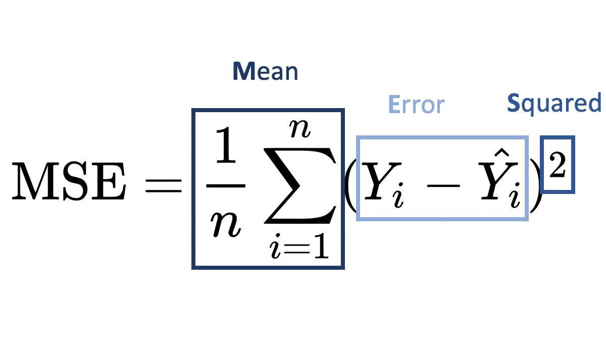
where:
- N is the number of data points in the node,
- yi is the target value for observation i,
- yˉ is the mean of the target values in that node.
Each possible split is evaluated by calculating the MSE for the left and right child nodes after the split. The best split minimizes the weighted average of the MSE of these child nodes:
MSE_split = (N_L / N) * MSE_L + (N_R / N) * MSE_R
where NL and NR are the sizes of the left and right child nodes, respectively.
b. Recursive Binary Splitting
Once the best split is determined, the data is divided into two subsets (left and right child nodes), and the process is repeated for each subset. This recursive binary splitting continues until a stopping criterion is met, such as:
- Maximum tree depth.
- Minimum number of samples in a node.
- Minimum reduction in error by further splitting.
3. Building the Tree: An Example with Simple Data
To illustrate the mechanics of a Decision Tree Regressor, let’s consider a small dataset with a single feature XXX and target variable yyy:
X = 1, 2, 3, 4, 5
Y = 2, 3, 4, 5, 6
The tree-building process would involve:
- Evaluating Splits: Consider potential split points within X (e.g., between values 1.5, 2.5, etc.).
- Calculating MSE: For each split point, compute MSE for the resulting subsets.
- Choosing the Split: Select the split with the lowest weighted MSE.
For instance, if splitting at X=2.5 gives the lowest MSE, it becomes the first split, creating left and right child nodes. This process continues recursively.
4. Key Parameters That Control Decision Tree Behavior
To prevent overfitting or underfitting, Decision Tree Regressors have key parameters that control the depth and structure of the tree:
- Max Depth: The maximum depth of the tree. Limits growth to avoid overfitting.
- Min Samples Split: The minimum number of samples required to consider a split at a node.
- Min Samples Leaf: The minimum number of samples required to be in a leaf node.
These parameters ensure the model generalizes better by controlling how deeply the data can be divided.
Certainly! Here’s an in-depth blog-style exploration of Decision Tree Regressor, breaking down each aspect of the model, its intuition, and application.
5. Advantages and Drawbacks
Advantages:
- Interpretability: Each decision path in the tree represents a clear set of rules.
- Non-linearity: Decision trees can capture complex relationships without requiring feature transformation.
- Feature Importance: Trees inherently provide information on feature importance.
Drawbacks:
- Overfitting: Deep trees can capture noise, leading to poor generalization.
- Instability: Small changes in data can lead to entirely different trees.
- Limited Smoothness: Predictions may not be as smooth as linear models.
6. Pruning: Avoiding Overfitting
Pruning is a technique used to remove sections of the tree that provide little predictive power, simplifying the model to prevent overfitting. Cost-complexity pruning (or post-pruning) is commonly applied, where the tree is grown fully, then branches are pruned back based on a threshold for error reduction.
This allows the model to keep only the most significant splits, ensuring a balance between complexity and generalization.
7. Applications and Use Cases
Decision Tree Regressors are suited for:
- Predicting housing prices: Accounting for location, size, and other non-linear factors.
- Estimating demand: Factoring in complex seasonality and external conditions.
- Stock market analysis: Capturing patterns in historical data that impact prices.
They’re also useful as base models in ensemble methods like Random Forests and Gradient Boosting, which aggregate multiple trees to reduce variance and improve accuracy.
8. A Walkthrough Example in Python
Using Python’s DecisionTreeRegressor from Scikit-learn, we can build a Decision Tree Regressor on the Boston Housing dataset:
from sklearn.tree import DecisionTreeRegressor
from sklearn.datasets import load_boston
from sklearn.model_selection import train_test_split
from sklearn.metrics import mean_squared_error
# Load dataset
data = load_boston()
X, y = data.data, data.target# Split data
X_train, X_test, y_train, y_test = train_test_split(X, y, test_size=0.2, random_state=42)# Instantiate and train model
tree_regressor = DecisionTreeRegressor(max_depth=4)
tree_regressor.fit(X_train, y_train)# Predictions and evaluation
y_pred = tree_regressor.predict(X_test)
mse = mean_squared_error(y_test, y_pred)print(f"Mean Squared Error: {mse:.2f}")
In this example, we limited the depth to prevent overfitting, achieving a reasonable trade-off between accuracy and complexity.
Certainly! Adding a section on dtreeviz provides a way to visualize and interpret the decision tree structure and splitting process, which enhances our understanding of how decision trees operate.
9. Visualizing Decision Tree Splits with dtreeviz
One of the most effective ways to understand a Decision Tree Regressor is to visualize its structure. dtreeviz is a Python library that provides an intuitive, visual representation of decision trees, showing detailed splits, decision rules, and even error distributions at each node. This can be particularly helpful for interpreting complex trees and gaining insights into how the model divides data at each step.
a. Installation and Setup
To get started with dtreeviz, install it using pip:
pip install dtreevizOnce installed, we can visualize our Decision Tree Regressor model on a sample dataset, such as the famous Iris dataset.
b. Visualizing a Decision Tree Regressor on the Iris Dataset
Let’s create a decision tree, fit it on the Iris dataset, and visualize it using dtreeviz. Although the Iris dataset is more commonly used for classification, this example will demonstrate how to use dtreeviz with a Decision Tree Regressor.
from sklearn.datasets import load_iris
from sklearn.tree import DecisionTreeRegressor
from dtreeviz.trees import dtreeviz
import matplotlib.pyplot as plt
# Load the Iris dataset
data = load_iris()
X = data.data[:, 2:] # Use petal length and width
y = data.data[:, 0] # Predict sepal length as a continuous variable# Fit the Decision Tree Regressor
regressor = DecisionTreeRegressor(max_depth=3)
regressor.fit(X, y)# Visualize the tree with dtreeviz
viz = dtreeviz(regressor, X, y,
feature_names=data.feature_names[2:],
target_name="sepal length",
title="Decision Tree Regressor on Iris Data")viz.view() # This will open an interactive window with tree visualization
c. Understanding the Visualization

With dtreeviz, we get a detailed graphical representation of the decision tree, highlighting:
- Split Conditions: Each node displays the feature and threshold used to make the split, allowing us to see which features are most influential in dividing the data at different tree depths.
- Error Reduction:
dtreevizshows histograms of target values in each node, providing insight into the distribution and error at each step. - Color Coding: The visualizer uses color coding to make the regression tree’s prediction boundaries and node distributions clearer. This is particularly helpful for understanding how the tree structure adapts to data patterns in non-linear regression tasks.
By examining these splits visually, we can see exactly how the tree makes decisions and reduces the error, step by step, in a clear and intuitive way. Visual tools like dtreeviz make interpreting decision trees much easier, turning a complex series of splits into an accessible, meaningful visualization.
Conclusion
Decision Tree Regressors are versatile and intuitive models that allow us to capture complex, non-linear relationships in data through a simple, rule-based approach. By recursively splitting the data into smaller and more homogeneous subsets, decision trees create a structured pathway for making predictions. While their interpretability and non-linear capabilities make them highly valuable, especially for small to medium datasets, they can be prone to overfitting without proper tuning or pruning. However, this limitation is often mitigated when they serve as building blocks in ensemble methods like Random Forests or Gradient Boosting, which boost their predictive power and generalization.