Essential Regression Evaluation Metrics: MSE, RMSE, MAE, R², and Adjusted R²

In regression analysis, evaluating model performance is essential for understanding how well the model fits the data. This post covers five important metrics for regression model evaluation: Mean Squared Error (MSE), Root Mean Squared Error (RMSE), Mean Absolute Error (MAE), R-squared (R²), and Adjusted R-squared. Each metric has its specific use cases, advantages, and limitations. Let’s break down each metric and see how it can be applied to model evaluation.
1. Mean Squared Error (MSE)
Definition: MSE is a common metric used to measure the average of the squared differences between predicted and actual values. It penalizes larger errors more severely, making it sensitive to outliers.
Formula:
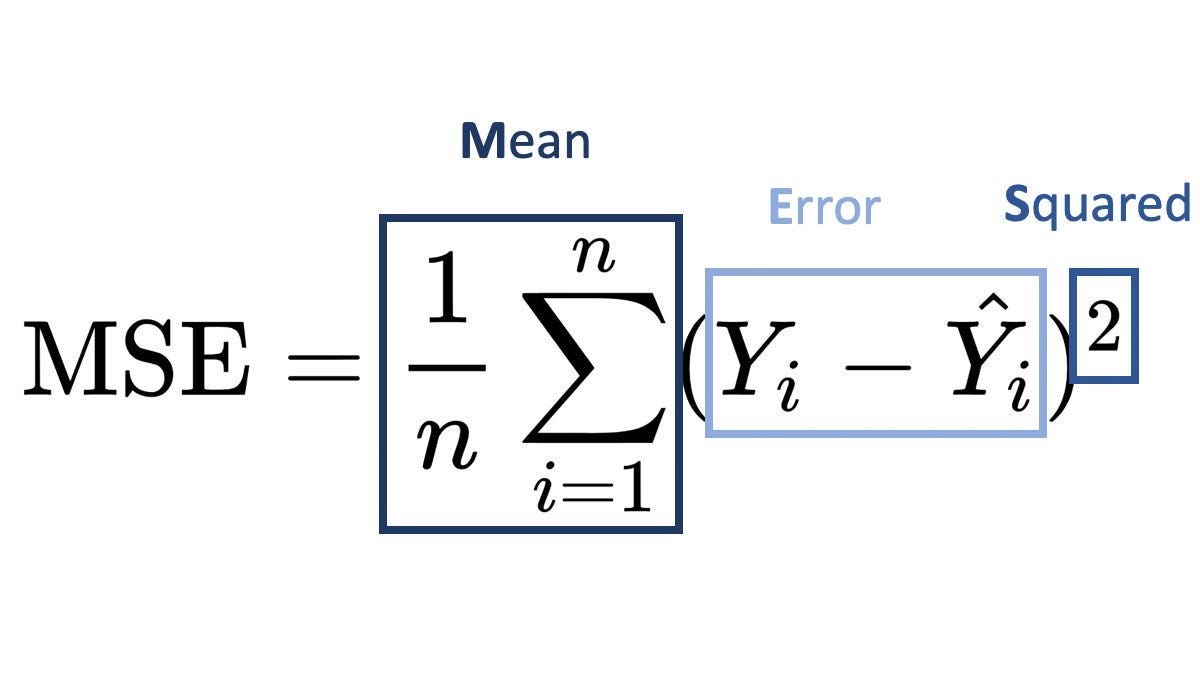
where:
- yi is the actual value,
- y^i is the predicted value,
- n is the number of data points.
Advantages:
- Emphasizes larger errors, making it useful when large errors are undesirable.
- Differentiable, so it’s commonly used in model optimization.
Disadvantages:
- Sensitive to outliers due to the squared term.
- Errors are squared, so the metric is not in the same unit as the target variable.
Code Example:
from sklearn.metrics import mean_squared_error# Define actual and predicted values
y_true = [11, 20, 19, 17, 10]
y_pred = [12, 18, 19, 18, 10]# Calculate MSE
mse = mean_squared_error(y_true, y_pred)
print("Mean Squared Error (MSE):", mse)
Interpretation: A lower MSE value indicates a better fit. Since MSE squares errors, even small differences are amplified, which can be helpful for identifying models with outliers.
2. Root Mean Squared Error (RMSE)
Definition: RMSE is the square root of MSE, bringing the metric back to the same units as the target variable. It provides an easily interpretable measure of average error size.
Formula:

Advantages:
- In the same units as the target variable, making interpretation more intuitive.
- Penalizes larger errors similarly to MSE.
Disadvantages:
- Still sensitive to outliers.
Code Example:
import numpy as np# Calculate RMSE
rmse = np.sqrt(mse)
print("Root Mean Squared Error (RMSE):", rmse)Interpretation: RMSE values closer to 0 indicate better model performance. RMSE’s interpretation is straightforward since it’s in the same units as the target variable.
3. Mean Absolute Error (MAE)
Definition: MAE measures the average magnitude of errors in predictions, without considering their direction. It’s calculated as the average of absolute differences between predicted and actual values.
Formula:

Advantages:
- Robust to outliers as it doesn’t square the errors.
- Easy to interpret as it represents the average error.
Disadvantages:
- May not penalize large errors as strongly as MSE or RMSE.
Code Example:
from sklearn.metrics import mean_absolute_error# Calculate MAE
mae = mean_absolute_error(y_true, y_pred)
print("Mean Absolute Error (MAE):", mae)Interpretation: MAE gives a direct idea of the average prediction error. Lower values of MAE indicate a better fit.
4. R-squared (R²)
Definition: R², or the coefficient of determination, indicates the proportion of the variance in the dependent variable that is predictable from the independent variables. It’s a measure of model fit.
Formula:

where:
- SSres = sum of squared residuals,
- SStot = total sum of squares.
Advantages:
- Intuitive interpretation: proportion of explained variance.
- Commonly used in linear regression.
Disadvantages:
- Does not penalize for the addition of irrelevant features.
- Not suitable for non-linear models.
Code Example:
from sklearn.metrics import r2_score# Calculate R²
r2 = r2_score(y_true, y_pred)
print("R-squared (R²):", r2)Interpretation: R² values closer to 1 indicate a better fit. A value of 1 means the model perfectly explains all the variance in the target variable.
5. Adjusted R-squared
Definition: Adjusted R² modifies R² to penalize adding irrelevant predictors to the model, making it more reliable for models with multiple predictors.
Formula:

where:
- n = number of observations,
- p = number of predictors.
Advantages:
- Adjusts for the number of predictors, making it suitable for multiple regression.
- Useful for comparing models with different numbers of predictors.
Disadvantages:
- More complex to calculate than R².
- May not be very informative for single-predictor models.
Code Example:
# Calculate Adjusted R²
n = len(y_true)  # number of observations
p = 1  # number of predictors (in simple linear regression, p=1)
adjusted_r2 = 1 - (1 - r2) * (n - 1) / (n - p - 1)
print("Adjusted R-squared:", adjusted_r2)Interpretation: Adjusted R² is preferred over R² for multiple regression as it penalizes unnecessary predictors, making it more reliable for evaluating
6. Mean Absolute Percentage Error (MAPE)
Definition: MAPE measures the average percentage error between actual and predicted values, providing a percentage-based accuracy measure. MAPE is particularly useful when you want to understand the model’s performance in terms of relative errors.
Formula:
MAPE = (1/n) * Σ (|y_i — ŷ_i| / y_i) * 100
where:
- yi is the actual value,
- y^i is the predicted value,
- n is the number of data points.
Advantages:
- MAPE is expressed in a percentage, making it easily interpretable for comparison across different datasets.
- Provides a relative measure of error, so it’s useful when the scale of the data varies widely.
Disadvantages:
- Sensitive to very small actual values, as they can inflate the percentage error significantly.
- Undefined when actual values are zero.
Code Example:
import numpy as np# Define actual and predicted values
y_true = [11, 20, 19, 17, 10]
y_pred = [12, 18, 19, 18, 10]# Calculate MAPE
mape = np.mean(np.abs((np.array(y_true) - np.array(y_pred)) / np.array(y_true))) * 100
print("Mean Absolute Percentage Error (MAPE):", mape)
Interpretation: MAPE provides a percentage error between predicted and actual values. For instance, if MAPE is 5%, it means the model predictions deviate on average by 5% from the actual values. Lower values of MAPE indicate better model accuracy in relative terms.complex models.
Key Takeaways
- MSE and RMSE are useful for penalizing large errors, making them suitable when large prediction errors are costly.
- MAE provides a straightforward average error, which is more robust to outliers.
- R² is a good measure of how well the model explains variance but doesn’t penalize for extra predictors.
- Adjusted R² is an improved version of R², accounting for the number of predictors, and is ideal for comparing models with different complexities.
- MAPE: Ideal for a relative error measure, providing insight into model performance as a percentage.
Conclusion: Choosing the Right Metric for Regression Evaluation
In the realm of regression analysis, selecting the appropriate evaluation metric is crucial for accurately assessing model performance. Each metric — Mean Squared Error (MSE), Root Mean Squared Error (RMSE), Mean Absolute Error (MAE), R-squared (R²), Adjusted R-squared, and Mean Absolute Percentage Error (MAPE) — serves a specific purpose and comes with its own strengths and weaknesses. By understanding these metrics, you can make informed decisions about model selection and improve the reliability of your predictions. Whether you prioritize error sensitivity, interpretability, or variance explanation, combining multiple metrics can offer a well-rounded view of your model’s effectiveness, ultimately leading to better data-driven outcomes.